[Please note that the following article — while it has been updated from our newsletter archives — may not reflect the latest software interface and plot graphics, but the original methodology and analysis steps remain applicable.]
Guest Submission - Harland MacKenzie, Dana Corporation
One of the keys to understanding how a system or component will react to conditions outside its validation envelope is the life-stressor slope. Generally, the useful life of a component decreases with increased levels of stress or "input." In essence, it comes down to developing a fatigue curve for a particular system then exploiting the design margin during testing. The hard part, quite often, is determining a confident estimate for the life-stressor slope; because even a small error results in predictions being quite far off. This article will examine some of the basics of accelerated life testing and some techniques to utilize the inverse power law to improve testing time, cost and life prediction accuracy.
What is Accelerated Life Testing?
Accelerated life testing (ALT) exploits the fatigue properties of materials to aid in the design and validation process. The general trend is to use ALT as a method to demonstrate the suitability of a particular design and/or system for field usage. But if all that is taken away is an estimate of useful life (or time to failure), the effort has been half wasted. Quite often, the failure mode is actually more valuable than the time to failure. If design changes can be made to eliminate or significantly delay the onset of the "first failure," great gains can be made in system reliability.
Accelerated testing is not about detecting PPM (parts per million) level faults. Most test programs run few parts, perhaps a dozen or fewer. Considering that the probability of finding a PPM level issue with 12 samples approaches the odds on some lotteries – the chance of success is low. That said, test conditions can be set up that occur rarely in the field (temperature extremes, for example) and therefore may be able to induce failure modes that are difficult to detect when testing within the design envelope.
Another useful application for the ALT data is to aid in determining the effect of operating a system outside its original design conditions. Generally, this allows the development of reasonably accurate estimates of life when operated at higher loads.
What is Stress?
Simply put, stress is anything that can cause a component or system to fail. Some of the obvious factors are:
- Mechanical loads (e.g., stress / strain / force)
- Hydrostatic / dynamic forces (e.g., pressure / wind loads)
- Temperature extremes and thermal shocks
- Vibration inputs (e.g., GRMS road load / engine vibration)
- Corrosive environments (e.g., sea water / road salt)
These are probably some of the first factors that come to mind when evaluating the "strength" of a particular design. But, depending on the usage and the material, just about anything can cause the system to degrade or fail prematurely, so one needs to keep an open mind when developing accelerated life tests.
In the field, unlike the lab where single stress testing is common, multiple stresses are quite often applied at the same time. The combination of multiple stresses can interact and essentially increase the effective stress applied. It is also possible to add in the lab stressors that are not present in the field to further speed up testing. The problem comes when it is time to determine the lab-field correlation, or how many hours in the field is equivalent to an hour on test.
One good example of this is in corrosion testing where acetic acid is added to the salt fog solution in SWAAT (ASTM G85 - Annex 3) type tests for automotive radiators. While the lower pH of the solution accelerates corrosion, outside of a few situations, little "salad dressing" is actually seen on the roads. In this case, much work is needed to relate the life of a component in the test chamber to that on the road. For this reason, it is generally better not to introduce artificial factors early in the development of an accelerated life test program or specification.
What is Life?
Life is basically any quantifiable measure of durability for a component or system. The end of life does not necessarily need to be the destruction of the component.
Understanding the failure criteria is a prerequisite for most testing. Obviously, if the component is in multiple barely recognizable pieces at the end of the test, failure will be easy to conclude. Many other cases can also be considered as failure; for example, if a frozen but not burst water pump will probably return to normal output when it thaws, does that constitute a failure?
It is important to have a firm grasp before testing starts as to what will be considered a failure and result in the termination of the test. Three principle types of failure to consider are:
- Hard Failure – the component ceases to function and does not return to usable status when the stress is removed. This is generally called a destructive failure. Example: A frozen and burst water pump.
- Soft Failure – the component ceases to function while the elevated stress is applied but returns to function at normal levels of stress. Example: A frozen but not burst water pump.
- Performance Failure – the component continues to function but at a reduced level of performance while the stress is applied. Performance may return to "normal" once the stress is removed but a permanent reduction in performance is also a possibility. Example: A water pump that functions but at a lower output.
It is important to keep the end user in mind when determining if an outcome is a failure. Something that is a concern to the design team may not be detected by the end user; so is it a failure? A good example of this is the failure of a single pixel in an LCD TV array – possibly an indication of design issues but probably unnoticed by someone watching the latest Hollywood release. Even if multiple pixels fail, they may not be noticed unless they are grouped together. It is important not to overestimate the sensitivity of end users to "engineering" failures.
In most components and just about all systems, there will be more than one failure mode possible. These failure modes may interact (mask or enhance each other), and are generally thought of as "competing" failure modes. In these cases, it is best to focus on the end user's experience. A very effective system model can be derived if all failure modes that lead to the same outcome are lumped together for analysis purposes. The motorist may not care about the details as to why the car will not start but will certainly notice when it does not.
Life-Stress Relationships
Generally speaking, the "life" of a component will go down as stress goes up. While this is not a hard and fast rule, very few systems do not behave in this intuitive fashion. This allows for shorter test times at higher levels of stress. With solid knowledge of the life-stressor relationship, effective predictions of life at normal or usage conditions can be made.
Probably the most important and widely used model for mechanical systems is the inverse power law (IPL).

The most critical factor is n, the life-stressor slope with s being stress applied to the system. A is a convenient mathematical constant; in reality it relates the basic mechanical strength of the design to resist the stress applied to it.
More generally, if multiple stressors need to be considered, the model is given by:

Since most fatigue testing generally fits a Weibull distribution, it may be best to consider the life being modeled as the mean or B10 life of the component.
An important measure often used in life testing is the acceleration factor (AF), which relates how one cycle or hour at an elevated stress level (S) relates to the usage, or base, level (SBase).

There are many other life-stress relationships that are commonly employed based on the underlying physics of failure. See references [1] and [3] for more information.
Inverse Power Law in Action
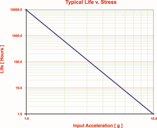
The practical application of the IPL allows "scaling," through the acceleration factor, of data and predictions from one stress level to another. In general, this is used to predict the life of a component at a stress level lower than was tested. The following plot depicts a typical IPL relationship (with a life – stress slope of 4) that could represent the life of a component or a full system. In general, the data are plotted using a log-log representation, with the stressor as the abscissa (horizontal axis) and the life as the ordinate (vertical axis).

With this example, if testing were conducted at 4 g of input acceleration, the expected life would be about 35 hours. This can be related back to a prediction at the operating conditions (1 g) to a life of about 10,000 hours. The acceleration factor is 256, or 1 hour at 4 g is equivalent to 256 hours at 1 g.
Basically, using this data, we can test any number of components to failure in a few days and get feedback about durability at base conditions without testing for 416+ days. In practice though, acceleration factors much above 100 can prove problematic by producing false failures that would not be seen in the field.
Adding Up Damage – Miner’s Rule
Most systems and components do not see constant stress input throughout their service lives. In most cases, there are low – high – low periods of loading. Likewise in testing, it may not be practical to always run at fixed levels of input. At lower levels, closer to field conditions, the time required to run until failure may be prohibitive. In these cases, it may be advantageous to "step" or increase the stress over time. The problem comes down to analyzing the resulting data and relating back to field or base conditions.
One way of dealing with these sorts of situations is to use a damage model. The foundation of most damage models is that each cycle or hour of stress exposure accumulates damage leading to eventual failure. One of the most popular, and easiest to interpret models is Miner’s rule.

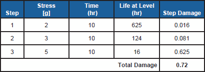
When applying Miner’s rule, each constant stress step accumulates damage based on the ratio of the duration of the step (Ni) to the life of the component if the whole test had been run at that level (Li). The failure point is predicted to occur when the total damage (DTotal – summed from each step) reaches unity. Using the slope and data model from the previous plot as a simple three-step example:

The total damage sums to 0.72 so the component would not be expected to fail. Another way of looking at the same data is that 30 hours of testing time (3 x 10 hour steps) would accumulate a similar amount of damage as if the unit had run for 425 hours at the lowest level of 2 g. This large acceleration factor comes from the sensitivity of the component to stress being quite significant – n is 4 in this example.
Obviously, this simple tool has limitations but it can be used surprisingly effectively to aid in developing test plans and in relating results of similar tests run at different levels. In general, not all samples in any given fatigue-based test will fail at the same time. Miner’s rule is probably best used to predict/ scale either B10 or mean life, much like working with the IPL.
Determining the IPL Slope
The three methods outlined next can be used to determine with reasonable accuracy the slope of the life-stressor line for a particular design or material.
1. IPL Slope from Datasheets
The easiest means of determining the life-stressor slope is to simply "look it up." For mechanical types of loads that translate into basic stress and strain in the base materials of the components, data from textbooks and datasheets can be used to give guidance. In general practice, S-N curves can be quite limited to generic materials and may not adequately represent the stress state of a component in use. While a significant data set is available for most metals, often little data will exist for other materials. In cases where data can be found, it most likely will not incorporate effects of mean stress and probably was determined through the use of bending or uniaxial tension on standard coupons.
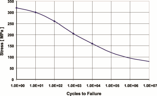
The following plot is representative of what is typically available from open literature. While we are interested in life- stress relationships, most of the data to be found is plotted in the "opposite" direction, as stress-life or S-N data.

The first problem one encounters with textbook data is that it generally covers a wide range of stress/strain conditions, from low cycle fatigue up to "infinite" life. Depending on the application of the system under investigation, choosing which portion of the data to use for your estimate can be critical.
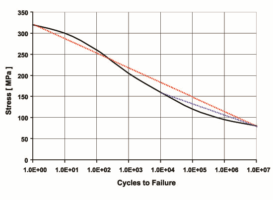
Because the life-stress slope is usually quite different in low cycle fatigue regions than in high, it is important to have an idea of the stress state (high vs. low) that the components will see during field use. Consider the plot shown next. There are many possible ways to fit a straight slope to the data for this plot; each will result in significant differences.

For example, if the whole range of the presented data is used (red line) that results in a S-N slope of about 0.08, which translates into a life-stress of n = 12. On the other hand if we know that the operational and test regime will be in the high cycle fatigue range then the blue line is a better choice from this data. With that assumption, a life-stress slope of about 10:1 is found. This is quite a large difference, especially when you recall that this is the exponent in the equation. Since very few systems are designed to survive only a few cycles, when in doubt bias the fit towards the lower stress, high cycle data.
It is best to use textbook data only as a starting point or for rough estimates. There are just too many factors at work for accurate predictions, even in non safety-critical systems.
2. IPL Slope from Material Testing
The second method for determining the life-stress slope is to perform simple experiments with samples of the actual material in use. This has the advantage of being able to closely resemble the stress state in the field and may be the only choice if "textbook" data is not available for the material of concern. One other advantage is that it presents the opportunity to gather data using field equivalent types of loads, such as GRMS values for vibration over a more generic mechanical stress. This may also be the only choice if the life-limiting stress is unconventional, such as the exposure of aluminum to mild acid solutions previous discussed.
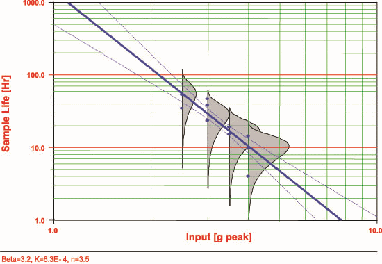
The following plot is based on data taken from an experiment with an aluminum brazing sheet used at Dana Corporation to make oil cooler brackets – little fatigue data existed for this material in post-brazed conditions. It was most expedient to construct a small series of tests with weighted strips of material attached to the shaker table – hence they were called the "flapping strip" experiments.

The experiment was quite simple. 10 coupons 6" long were mounted vertically on a shaker table and a sine sweep from 10 – 100 Hz was performed. Four levels of input were used from 2.5 up to 4 gPeak. These levels and the frequencies involved do not differ much from some of the inputs seen from actual road load testing of full cooler systems.
Due to the abstract nature of the experiment, little more than the slope of the life-stress line (3.5 in this case) is of value in future designs and testing analysis. One interesting observation is that if textbook data had been used to estimate the slope for this material, a slope of closer to 10 would have been found – a great deal different than what the experiments showed. Had the higher estimate been used, gross errors in predictions would have been made that could have led to debate on the validity of the test, or worse, the suitability of the component. The investment of a day or so in effort to organize and a couple days of shaker time was well worth the results.
3. IPL Slope from System Testing
The final method to determine the life-stressor relationship is to perform system or sub-system level testing. This tends to be the most costly and time-consuming method but also produces data that most closely represents field usage.
If the components have a significant design margin (especially a safety-critical item) then running at operation conditions may be impractically long but unfortunately provides the most useful data point. Working with components as close as possible to production design generally produces results and uses inputs that most closely resemble field conditions.
The inputs and outputs do not need to be abstract concepts such as stress and strain, but rather engineering and user inputs such as temperature, button pushes, speeds and on-off-on cycles. Having easy-to-interpret results, such as hours or days to failure, also helps in relating testing and predictions to full system analysis and field conditions.
Some tips to consider for system testing:
- You can never have too much data. Run at least two samples at a minimum of three different stress levels. Run at least one set as close to the field conditions as possible, even if you do not have time to run to failure. Bias your samples towards the end of the range. For more, see [1].
- Run all samples to failure. The added information from failure analysis is quite valuable for future designs. This not only aids in understanding of failure modes but working towards eliminating those failures also generally improves the reliability and durability of the product.
- Watch for failure mode switches at higher input levels. This might be a sign that you have exceeded reasonable limits of testing or switched to a low cycle fatigue regime. It is important to be careful not to induce foolish failures – use common sense when examining results and developing testing levels. If a failure mode that is impossible to occur in the field is forced, what truly is gained in the exercise?
- Work with multiple levels of fixed stress. Each component should only see one stress level during the test. While it is possible to use Miner’s rule to help analyze step-stress or variable stress testing, it adds another level of analysis in determining the life-stressor slope.
As pointed out above, the switch from high to low cycle fatigue can be problematic and represents the practical upper limit of acceleration that can be achieved. In general, the switch is not a clear cut-off point but a gradual transition. Thus, it is important to look for signs of this transition in data.
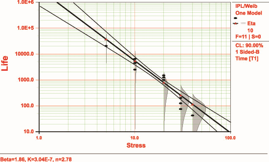
The first plot below comes from a case study into the durability of an oil cooler exposed to cyclical pressure. In this analysis, if all the data points are considered to fit one model, a life-stress slope of ~ 2.8 is found. It is apparent that not all of the data, especially at the limits, fits the model very well.

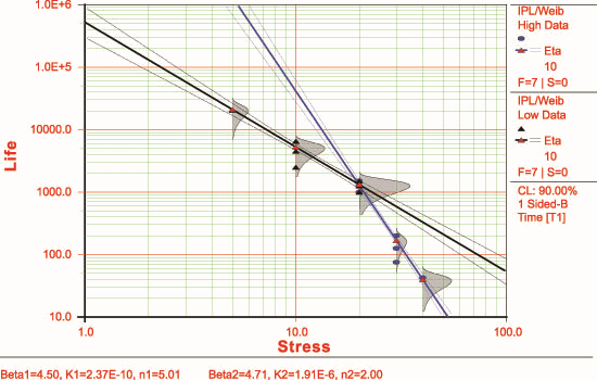
The second plot is the same data set but broken into two sections, a high and low stress regime. The data set fits a high-low model much better. The key is to understand where the operating point of the system lies to choose which model, the low (n = 2) or the high stress model, where there is more sensitivity to stress.

Recommendations
Accelerated life testing can save time and cost during the design and development validation phase in many industries. With little effort, basic life-stressor models can be developed using the inverse power law model. Having a firm grasp on the sensitivities to exposure at different levels of field stresses is a valuable tool to assess suitability to "off-design" conditions. This can then be used to explore sensitivity of a system to its "inputs" – and thereby develop more robust components.
References
[1] W. B. Nelson. Accelerated Testing: Statistical Models, Test Plans, and Data Analysis, USA: Wiley-Interscience, 1990.
[2] H. W. McLean. HALT, HASS & HASA Explained, USA: ASQ Quality Press, 2000.
[3] ReliaSoft. Accelerated Life Testing Reference, Tucson, AZ: ReliaSoft Publishing, 2007.
About the Author
Harland MacKenzie is the reliability manager for Dana Power Technologies in Oakville, Ontario. He acts as a resource to the company in areas of testing, reliability and statistics. His primary interests are centered around using and developing techniques to improve design and development testing, with a focus on improving product performance and reducing warranty cost. Harland has presented at several Applied Reliability Symposium (ARS) conferences over the past several years on the subject of accelerated life testing. He also teaches courses within Dana and has several publications in the area of testing and specification development for automotive components and systems. He can be reached at [email protected].


