[Please note that the following article — while it has been updated from our newsletter archives — may not reflect the latest software interface and plot graphics, but the original methodology and analysis steps remain applicable.]
Software Used: Lambda Predict, Weibull++, ALTA
In today's competitive electronic products market, having higher reliability than competitors is one of the key factors for success. To obtain high product reliability, consideration of reliability issues should be integrated from the very beginning of the design phase. This leads to the concept of reliability prediction. Historically, this term has been used to denote the process of applying mathematical models and component data for the purpose of estimating the field reliability of a system before failure data are available for the system. However, the objective of reliability prediction is not limited to predicting whether reliability goals, such as MTBF, can be reached. It can also be used for:
- Identifying potential design weaknesses
- Evaluating the feasibility of a design
- Comparing different designs and life-cycle costs
- Providing models for system reliability/availability analysis
- Establishing goals for reliability tests
- Aiding in business decisions such as budget allocation and scheduling
Once the prototype of a product is available, lab tests can be utilized to obtain more accurate reliability predictions. Accurate prediction of the reliability of electronic products requires knowledge of the components, the design, the manufacturing process and the expected operating conditions. Several different approaches have been developed to achieve the reliability prediction of electronic systems and components. Each approach has its unique advantages and disadvantages. Among these approaches, three main categories are often used within government and industry: empirical (standards based), physics of failure and life testing. In this article, we will provide an overview of all three approaches.
First, we will discuss empirical prediction methods, which are based on the experiences of engineers and on historical data. Standards, such as MIL-HDBK-217 and Bellcore/Telcordia, are widely used for reliability prediction of electronic products. Next, we will discuss physics of failure methods, which are based on root-cause analysis of failure mechanisms, failure modes and stresses. This approach is based upon an understanding of the physical properties of the materials, operation processes and technologies used in the design. Finally, we will discuss life testing methods, which are used to determine reliability by testing a relatively large number of samples at their specified operation stresses or higher stresses and using statistical models to analyze the data.
Empirical (or Standards Based) Prediction Methods
Empirical prediction methods are based on models developed from statistical curve fitting of historical failure data, which may have been collected in the field, in-house or from manufacturers. These methods tend to present good estimates of reliability for similar or slightly modified parts. Some parameters in the curve function can be modified by integrating engineering knowledge. The assumption is made that system or equipment failure causes are inherently linked to components whose failures are independent of each other. There are many different empirical methods that have been created for specific applications. Some have gained popularity within industry in the past three decades. The table below lists some of the available prediction standards and the following sections describe two of the most commonly used methods in a bit more detail.
| Prediction Method |
Applied Industry |
Last Update |
| MIL-HDBK-217F and Notice 1 and 2 |
Military |
1995 |
| Bellcore/Telcordia |
Telecom |
2011 |
| NSWC |
Mechanical |
2011 |
| FIDES |
Commercial/French Military |
2009 |
MIL-HDBK-217 Predictive Method
MIL-HDBK-217 is very well known in military and commercial industries. It is probably the most internationally recognized empirical prediction method, by far. The latest version is MIL-HDBK-217F, which was released in 1991 and had two revisions: Notice 1 in 1992 and Notice 2 in 1995.
The MIL-HDBK-217 predictive method consists of two parts; one is known as the parts count method and the other is called the part stress method [1]. The parts count method assumes typical operating conditions of part complexity, ambient temperature, various electrical stresses, operation mode and environment (called reference conditions). The failure rate for a part under the reference conditions is calculated as:
where:
- λref is the failure rate under the reference conditions
- i is the number of parts
Since the parts may not operate under the reference conditions, the real operating conditions will result in failure rates that are different from those given by the "parts count" method. Therefore, the part stress method requires the specific part’s complexity, application stresses, environmental factors, etc. (called Pi factors). For example, MIL-HDBK-217 provides many environmental conditions (expressed as πE) ranging from "ground benign" to "cannon launch." The standard also provides multi-level quality specifications (expressed as πQ). The failure rate for parts under specific operating conditions can be calculated as:
where:
- πS is the stress factor
- πT is the temperature factor
- πE is the environment factor
- πQ is the quality factor
- πA is the adjustment factor
Figure 1 shows an example using the MIL-HDBK-217 method (in ReliaSoft Lambda Predict software) to predict the failure rate of a ceramic capacitor. According to the handbook, the failure rate of a commercial ceramic capacitor of 0.00068 μF capacitance with 80% operation voltage, working under 30 degrees ambient temperature and "ground benign" environment is 0.0217 / 106 hours. The corresponding MTBF (mean time before failure) or MTTF (mean time to failure) is estimated to be 4.6140 / 107 hours.
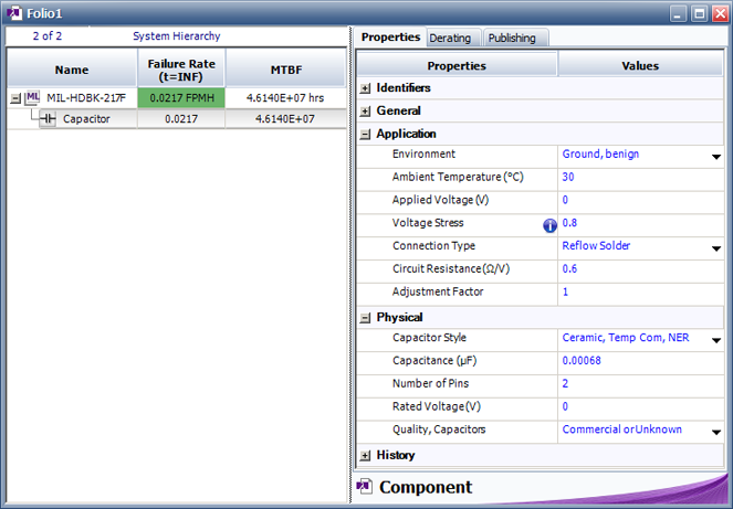
Figure 1: MIL-HDBK-217 capacitor failure rate example
Bellcore/Telcordia Predictive Method
Bellcore was a telecommunications research and development company that provided joint R&D and standards setting for AT&T and its co-owners. Because of dissatisfaction with military handbook methods for their commercial products, Bellcore designed its own reliability prediction standard for commercial telecommunication products. In 1997, the company was acquired by Science Applications International Corporation (SAIC) and the company's name was changed to Telcordia. Telcordia continues to revise and update the standard. The latest two updates are SR-332 Issue 2 (September 2006) and SR-332 Issue 3 (January 2011), both called "Reliability Prediction Procedure for Electronic Equipment."
The Bellcore/Telcordia standard assumes a serial model for electronic parts and it addresses failure rates at the infant mortality stage and at the steady-state stage with Methods I, II and III [2-3]. Method I is similar to the MIL-HDBK-217F parts count and part stress methods. The standard provides the generic failure rates and three part stress factors: device quality factor (πQ), electrical stress factor (πS) and temperature stress factor (T). Method II is based on combining Method I predictions with data from laboratory tests performed in accordance with specific SR-332 criteria. Method III is a statistical prediction of failure rate based on field tracking data collected in accordance with specific SR-332 criteria. In Method III, the predicted failure rate is a weighted average of the generic steady-state failure rate and the field failure rate.
Figure 2 shows an example in Lambda Predict using SR-332 Issue 3 to predict the failure rate of the same capacitor in the previous MIL-HDBK-217 example (shown in Figure 1). The failure rate is 9.655 Fits, which is 9.655 / 109 hours. In order to compare the predicted results from MIL-HBK-217 and Bellcore SR-332, we must convert the failure rate to the same units. 9.655 Fits is 0.0009655 / 106 hours. So the result of 0.0217 / 106 hours in MIL-HDBK-217 is much higher than the result in Bellcore/Telcordia SR-332. There are reasons for this variation. First, MIL-HDBK-217 is a standard used in the military so it is more conservative than the commercial standard. Second, the underlying methods are different and more factors that may affect the failure rate are considered in MIL-HDBK-217.
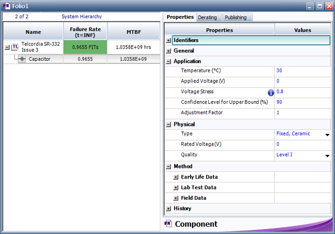
Figure 2: Bellcore capacitor failure rate example
Discussion of Empirical Methods
Although empirical prediction standards have been used for many years, it is always wise to use them with caution. The advantages and disadvantages of empirical methods have been discussed a lot in the past three decades. A brief summary from the publications in industry, military and academia is presented next [5-9].
Advantages of empirical methods:
- Easy to use, and a lot of component models exist
- Relatively good performance as indicators of inherent reliability
- Provide an approximation of field failure rates
Disadvantages of empirical methods:
- A large part of the data used by the traditional models is out-of-date
- Failure of the components is not always due to component-intrinsic mechanisms but can be caused by the system design
- The reliability prediction models are based on industry-average values of failure rate, which are neither vendor-specific nor device-specific
- It is hard to collect good quality field and manufacturing data, which are needed to define the adjustment factors, such as the Pi factors in MIL-HDBK-217
Physics of Failure Methods
In contrast to empirical reliability prediction methods, which are based on the statistical analysis of historical failure data, a physics of failure approach is based on the understanding of the failure mechanism and applying the physics of failure model to the data. Several popularly used models are discussed next.
Arrhenius's Law
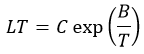
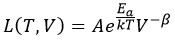
One of the earliest and most successful acceleration models predicts how the time-to-failure of a system varies with temperature. This empirically based model is known as the Arrhenius equation. Generally, chemical reactions can be accelerated by increasing the system temperature. Since it is a chemical process, the aging of a capacitor (such as an electrolytic capacitor) is accelerated by increasing the operating temperature. The model takes the following form.
where:
- L(T ) is the life characteristic related to temperature
- A is the scaling factor
- Ea is the activation energy
- k is the Boltzmann constant
- T is the temperature.
Eyring and Other Models
While the Arrhenius model emphasizes the dependency of reactions on temperature, the Eyring model is commonly used for demonstrating the dependency of reactions on stress factors other than temperature, such as mechanical stress, humidity or voltage.
The standard equation for the Eyring model [10] is as follows:
where:
- L(T ,S) is the life characteristic related to temperature and another stress
- A, α, B and C are constants
- S is a stress factor other than temperature
- T is absolute temperature
According to different physics of failure mechanisms, one more term (i.e., stress) can be either removed or added to the above standard Eyring model. Several models are similar to the standard Eyring model. They are:
Two Temperature/Voltage Model:
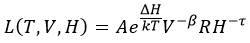
Three Stress Model (Temperature-Voltage-Humidity):
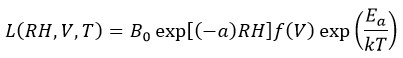
Corrosion Model:
Electronic devices with aluminum or aluminum alloy with small percentages of copper and silicon metallization are subject to corrosion failures and therefore can be described with the following model [11]:
where:
- B0 is an arbitrary scale factor
- α is equal to 0.1 to 0.15 per % RH
- f(V) is an unknown function of applied voltage, with empirical value of 0.12 to 0.15
Hot Carrier Injection Model:
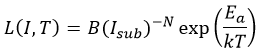
Hot carrier injection describes the phenomena observed in MOSFETs by which the carrier gains sufficient energy to be injected into the gate oxide, generate interface or bulk oxide defects and degrade MOSFETs characteristics such as threshold voltage, transconductance, etc. [11]:
For n-channel devices, the model is given by:
where:
- B is an arbitrary scale factor
- Isub is the peak substrate current during stressing
- N is equal to a value from 2 to 4, typically 3
- Ea is equal to -0.1eV to -0.2eV
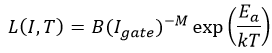
For p-channel devices, the model is given by:
where:
- B is an arbitrary scale factor
- Igate is the peak gate current during stressing
- M is equal to a value from 2 to 4
- Ea is equal to -0.1eV to -0.2eV
Since electronic products usually have a long time period of useful life (i.e., the constant line of the bathtub curve) and can often be modeled using an exponential distribution, the life characteristics in the above physics of failure models can be replaced by MTBF (i.e., the life characteristic in the exponential distribution). However, if you think your products do not exhibit a constant failure rate and therefore cannot be described by an exponential distribution, the life characteristic usually will not be the MTBF. For example, for the Weibull distribution, the life characteristic is the scale parameter eta and for the lognormal distribution, it is the log mean.
Black Model for Electromigration
Electromigration is a failure mechanism that results from the transfer of momentum from the electrons, which move in the applied electric field, to the ions, which make up the lattice of the interconnect material. The most common failure mode is "conductor open." With the decreased structure of Integrated Circuits (ICs), the increased current density makes this failure mechanism very important in IC reliability.
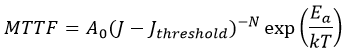
At the end of the 1960s, J. R. Black developed an empirical model to estimate the MTTF of a wire, taking electromigration into consideration, which is now generally known as the Black model. The Black model employs external heating and increased current density and is given by:
where:
- A0 is a constant based on the cross-sectional area of the interconnect
- J is the current density
- Jthreshold is the threshold current density
- E a is the activation energy
- k is the Boltzmann constant
- T is the temperature
- N is a scaling factor
The current density (J) and temperature (T) are factors in the design process that affect electromigration. Numerous experiments with different stress conditions have been reported in the literature, where the values have been reported in the range between 2 and 3.3 for N, and 0.5 to 1.1eV for Ea. Usually, the lower the values, the more conservative the estimation.
Coffin-Manson Model for Fatigue
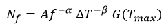
Fatigue failures can occur in electronic devices due to temperature cycling and thermal shock. Permanent damage accumulates each time the device experiences a normal power-up and power-down cycle. These switch cycles can induce cyclical stress that tends to weaken materials and may cause several different types of failures, such as dielectric/thin-film cracking, lifted bonds, solder fatigue, etc. A model known as the (modified) Coffin-Manson model has been used successfully to model crack growth in solder due to repeated temperature cycling as the device is switched on and off. This model takes the form [9]:
where:
- Nf is the number of cycles to failure
- Α is a coefficient
- f is the cycling frequency
- ΔT is the temperature range during a cycle
- Α is the cycling frequency exponent
- Α is the temperature exponent
- G(Tmax) is equal to:
which is an Arrhenius term evaluated at the maximum temperature in each cycle.
Three factors are usually considered for testing: maximum temperature (Tmax), temperature range (ΔT) and cycling frequency (f). The activation energy is usually related to certain failure mechanisms and failure modes, and can be determined by correlating thermal cycling test data and the Coffin-Manson model.
Discussion of Physics of Failure Methods
A given electronic component will have multiple failure modes and the component's failure rate is equal to the sum of the failure rates of all modes (i.e., humidity, voltage, temperature, thermal cycling and so on). The system's failure rate is equal to the sum of the failure rates of the components involved. In using the above models, the model parameters can be determined from the design specifications or operating conditions. If the parameters cannot be determined without conducting a test, the failure data obtained from the test can be used to get the model parameters. Software products such as ReliaSoft ALTA can help you analyze the failure data.
We will give an example of using ALTA to analyze the Arrhenius model. For this example, the life of an electronic component is considered to be affected by temperature. The component is tested under temperatures of 406, 416 and 426 Kelvin. The usage temperature level is 400 Kelvin. The Arrhenius model and the Weibull distribution are used to analyze the failure data in ALTA. Figure 4 shows the data and calculated parameters. Figure 5 shows the reliability plot and the estimated B10 life at the usage temperature level.
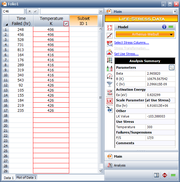
Figure 4: Data and analysis results in ALTA with the Arrhenius-Weibull model
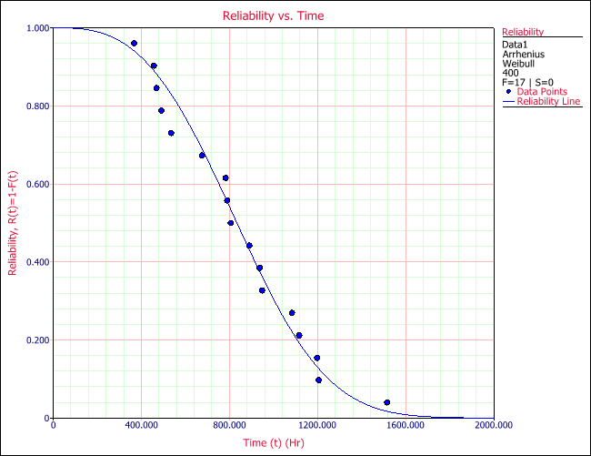

Figure 5: Reliability vs. Time plot and calculated B10 life
From Figure 4, we can see that the estimated activation energy in the Arrhenius model is 0.92. Note that, in ALTA, the Arrhenius model is simplified to a form of:
Using this equation, the parameters B and C calculated by ALTA can easily be transformed to the parameters described above for the Arrhenius relationship.
Advantages of physics of failure methods:
- Accurate prediction of wearout using known failure mechanisms
- Modeling of potential failure mechanisms based on the physics of failure
- During the design process, the variability of each design parameter can be determined
Disadvantages of physics of failure methods:
- Need detailed component manufacturing information (such as material, process and design data)
- Analysis is complex and could be costly to apply
- It is difficult to assess the entire system
Life Testing Method
As mentioned above, time-to-failure data from life testing may be incorporated into some of the empirical prediction standards (i.e., Bellcore/Telcordia Method II) and may also be necessary to estimate the parameters for some of the physics of failure models. However, in this section of the article, we are using the term life testing method to refer specifically to a third type of approach for predicting the reliability of electronic products. With this method, a test is conducted on a sufficiently large sample of units operating under normal usage conditions. Times-to-failure are recorded and then analyzed with an appropriate statistical distribution in order to estimate reliability metrics such as the B10 life. This type of analysis is often referred to as Life Data Analysis or Weibull Analysis.
ReliaSoft Weibull++ software is a tool for conducting life data analysis. As an example, suppose that an IC board is tested in the lab and the failure data are recorded. Figure 6 shows the data entered into Weibull++ and analyzed with the 2-parameter Weibull lifetime distribution, while Figure 7 shows the Reliability vs. Time plot and the calculated B10 life for the analysis.

Figure 6: Data and analysis results in Weibull++ with the Weibull distribution
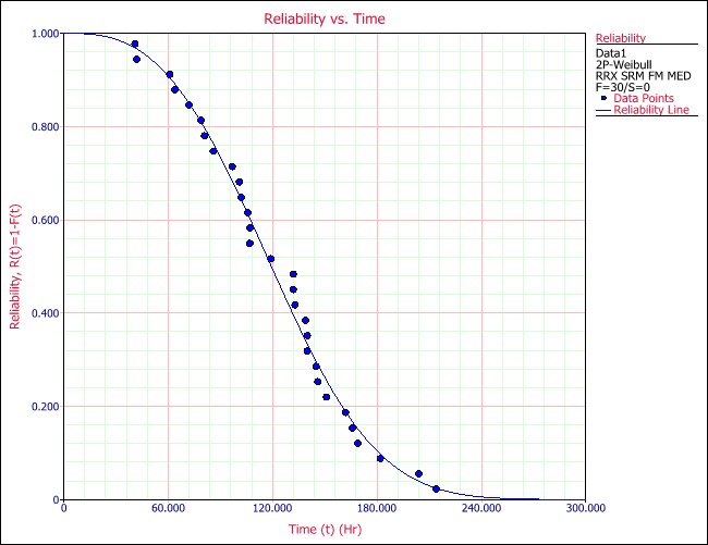
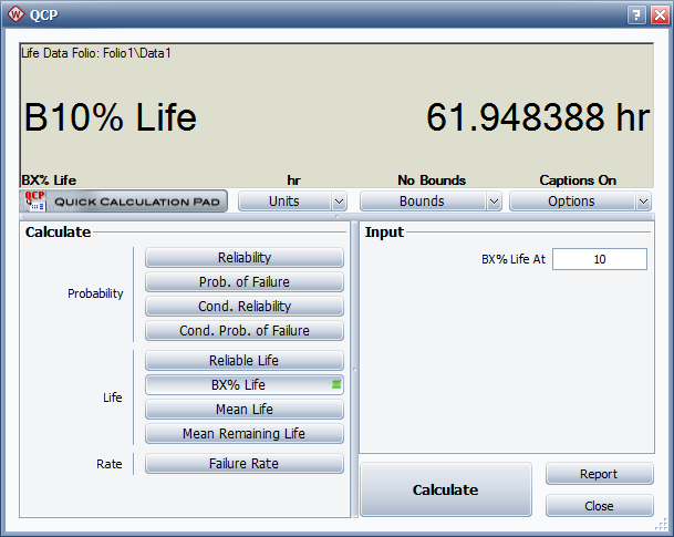
Figure 7: Reliability vs. Time plot and calculated B10 life for the analysis
Discussion of the Life Testing Method
The life testing method can provide more information about the product than the empirical prediction standards. Therefore, the prediction is usually more accurate, given that enough samples are used in the testing.
The life testing method may also be preferred over both the empirical and physics of failure methods when it is necessary to obtain realistic predictions at the system (rather than component) level. This is because the empirical and physics of failure methods calculate the system failure rate based on the predictions for the components (e.g., using the sum of the component failure rates if the system is considered to be a serial configuration). This assumes that there are no interaction failures between the components but, in reality, due to the design or manufacturing, components are not independent. (For example, if the fan is broken in your laptop, the CPU will fail faster because of the high temperature.) Therefore, in order to consider the complexity of the entire system, life tests can be conducted at the system level, treating the system as a "black box," and the system reliability can be predicted based on the obtained failure data.
Conclusions
In this article, we discussed three approaches for electronic reliability prediction. The empirical (or standards based) methods can be used in the design stage to quickly obtain a rough estimation of product reliability. The physics of failure and life testing methods can be used in both design and production stages. In physics of failure approaches, the model parameters can be determined from design specs or from test data. On the other hand, with the life testing method, since the failure data from your own particular products are obtained, the prediction results usually are more accurate than those from a general standard or model.
References
[1] MIL-HDBK-217F, Reliability Prediction of Electronic Equipment, 1991. Notice 1 (1992) and Notice 2 (1995).
[2] SR-332, Issue 1, Reliability Prediction Procedure for Electronic Equipment, Telcordia, May 2001.
[3] SR-332, Issue 2, Reliability Prediction Procedure for Electronic Equipment, Telcordia, September 2006.
[4] ITEM Software and ReliaSoft, D490 Course Notes: Introduction to Standards Based Reliability Prediction and Lambda Predict, 2015.
[5] B. Foucher, J. Boullie, B. Meslet and D. Das, "A Review of Reliability Prediction Methods for Electronic Devices," Microelectron. Wearout., vol. 42, no. 8, August 2002, pp. 1155-1162.
[6] M. Pecht, D. Das and A. Ramarkrishnan, "The IEEE Standards on Reliability Program and Reliability Prediction Methods for Electronic Equipment," Microelectron. Wearout., vol. 42, 2002, pp. 1259-1266.
[7] M. Talmor and S. Arueti, "Reliability Prediction: The Turnover Point," 1997 Proc. Ann. Reliability and Maintainability Symp., 1997, pp. 254-262.
[8] W. Denson, "The History of Reliability Prediction," IEEE Trans. On Reliability, vol. 47, no. 3-SP, September 1998.
[9] D. Hirschmann, D. Tissen, S. Schroder and R.W. de Doncker, "Reliability Prediction for Inverters in Hybrid Electrical Vehicles," IEEE Trans. on Power Electronics, vol. 22, no. 6, November 2007, pp. 2511-2517.
[10] NIST Information Technology Library. [Online document] Available HTTP: www.itl.nist.gov
[11] Semiconductor Device Reliability Failure Models. [Online document] Available HTTP: www.sematech.org/docubase/document/3955axfr.pdf